ISSN 2379-5980 (online) DOI 10.5195/LEDGER.2024.312

RESEARCH ARTICLE

Granger-Causal Effects of Consumer Behavior on NFT Sales

Stoyan R. Angelov*

Abstract. An understanding of what influences the NFT market is valuable in such a speculative space, and predictors of directional shifts in NFT sales are beneficial to NFT users and investors alike. For these reasons, research was undertaken to determine if metrics relating to consumer behavior could predict NFT market sales. To begin, a Buyer Activity Metric and a Buyer Valuation Metric were calculated using open-access data regarding the NFT market. A three-variable vector autoregression (VAR) model was then constructed using these metrics and NFT sales data. Changes in monthly NFT sales were found to be Granger-caused by changes in both the Buyer Activity Metric and the Buyer Valuation Metric. Changes in each metric were determined to precede changes in NFT sales by up to four months. The associations were also determined to be unidirectional, indicating a clear cause-and-effect style relationship. Questions about these predictive abilities were then theoretically explored.

*S. R. Angelov (stoyan.angelov@stern.nyu.edu) is studying Finance and Mathematics at NYU Stern.

1. Introduction

   The Non-Fungible Token (NFT) market has experienced significant changes in demand over the past years. Blockchain assets became extremely popular due to intense media coverage, celebrity endorsement, and the premise of the new technology itself during 2021.1 However, NonFungible.com’s Quarterly NFT Market Reports state that the total amount (USD) of NFTs traded declined by 77% between Q2-Q3 of 2022 alone, with Q1 and Q2 of 2022 also suffering severe losses in sales compared to previous quarters.2 Such fluctuations in sales have given rise to questions regarding influential factors in the NFT market. Questions of special consideration relate to how consumer activity impacts the vitality of the market as a whole, seeing as how total NFT market sales have taken drastic increases and decreases over relatively short periods of time. Resultingly, this paper aims to reveal the degree to which consumer behavior can forecast the total sales in the NFT market. To this end, two different metrics were calculated using multiple types of NFT market data. These metrics were tested alongside NFT sales data to determine any possible relationships. Specifically, Granger-causality hypothesis tests, based on a vector autoregression model, were used to evaluate the predictive abilities of the metrics.

   An investigation into the delayed effects of NFT consumer behavior improves users’ understanding of the market. It also may yield practical implications. For example, it is important for NFT investors to know whether the behavior of the average consumer can forecast the overall market’s sales. If directional changes in total NFT sales may be attributed to shifting consumer sentiment months in advance, investors may time their entrance into the NFT market accordingly. Researching the impacts of changing consumer sentiment also reveals more topics of inquiry worth studying. These topics include the impact that “whales” have on the NFT market and the holding times of the most expensive and influential NFT projects. Judging by fluctuations in NFT sales over recent years (in addition to other statistical measures), the NFT market is also heavily dictated by trends. If consumer behaviors can indicate when these trends begin, the origins of these behaviors certainly merit more investigation.

   Extreme volatility in sales is an intrinsic characteristic of the NFT market. This is because NFT investing is a highly speculative industry—returns depend greatly on the amount of public attention that individual projects receive.3 As previously mentioned, it should not come as a surprise that fluctuations in NFT sales have been historically and haphazardly drastic. However, by investigating how the behavior of the average NFT consumer affects future NFT sales and market vitality, a seemingly unpredictable aspect of the market becomes more transparent.

   
   

2. Background on NFTs and Relevance to Existing Literature

   A Non-Fungible Token is a digital token, signifying a unit of value, available on a cryptocurrency blockchain (such as Ethereum, Solana, or WAX). These tokens are transactable through the smart contracts of the blockchain. Some key terms are defined below.

   • Blockchains: Distributed and decentralized databases that hold data records which validate Non-Fungible Token. This allows for cryptographic assets to be uniquely identified, connected, and ensured using cryptographic protocols.4

   • Smart Contracts: Programs that use Turing-complete scripting languages to administer complicated functions, enabling state transition replication over other consensus algorithms. Smart contracts highlight a consistency in transactions between parties and constitute the decentralized third party which allows for the fair and safe transaction between unfamiliar cryptocurrency wallet addresses.

   
   

   NFTs themselves—in common parlance meaning the digital property validated by the Non- Fungible Token, rather than the token itself—are unique individual assets. Unlike cryptocurrencies, “they cannot be exchanged like-for-like… making [them] suitable for identifying something or someone in a unique way,” as Wang et al. explain.5 Furthermore, the existence and ownership of NFTs are provable through their smart contracts on blockchains such as Ethereum. Smart contracts and the underlying code of a Non-Fungible Token also make viewing and recording the full trading history of NFTs quite simple, allowing for features such as indefinite trading royalties for the creators of NFTs.

   As Taherdoost highlighted in “Non-Fungible Tokens (NFT): A Systematic Review,” a concern arises in whether a standard methodology exists for determining an NFT’s value.6 Indeed, the unique nature of NFTs makes it very difficult to standardize pricing and has implicitly led to the aforementioned volatility in market value. In an effort to better understand fluctuations in market value, this study aims to uncover econometric predictors for the NFT market’s sales. Of course, forecasting trends in the NFT market is not a new area of research. Nadini et al. found that the daily sale prices of NFTs across virtually every category can be strongly predicted by the prices of the previous day using a simple least-squares regression (R2adj ≈ 0.5).7 It should be noted that these findings somewhat corroborate the highly positive autocorrelation found amongst timeseries data on NFT sales (as seen in the subsequent “Data and Methodology” section of this paper). This degree of autocorrelation formed the methodological justification of this study, so this paper comes as a natural evolution to the findings of Nadini et al. Where this paper differs from its predecessor is in its attempt to find predictors of longer-term trends in NFT market sales, not daily movements in aggregate NFT prices. Furthermore, it is novel in its choice of independent variables and statistical frameworks used.

   
   

3. Data and Methodology

   The dataset used for analysis was constructed using open-access data available on the NFT data aggregator CryptoSlam.8 CryptoSlam scrapes its data directly from the Ethereum, WAX, and Flow blockchains. WAX and Flow are blockchains that are specifically designed for digital asset creation and trading. All of CryptoSlam’s data are recorded from on-chain activity and include activity from NFT marketplaces such as OpenSea. For this paper, monthly data regarding transactions, number of buyers, and total sales in the market (USD) between July 2017 and March 2023 were collected. The data was collected directly from the monthly CryptoSlam NFT Global Sales Volume webpage, 9 and the resulting dataset of 69 observations per variable was used for all data manipulation and statistical analysis.

   The data were aggregated at the monthly level, as opposed to a more granular timeframe, for several reasons. Most importantly, the monthly time frame best suits the scope of the study, as it was concerned with predicting sustained, longer-term trends in the NFT market’s sales. Additionally, analyzing monthly data helped filter out white noise from the dataset which may have clouded the ensuing statistical analysis. This decision reduced the effect which intra-month volatility might have had on the Vector Autoregression model and subsequent Granger-causal hypothesis tests. Furthermore, the monthly timeframe smoothed the sudden, sharp, and often one-day swings in activity motivated by single NFT collections. These swings would have needed some form of filtering before statistical analysis if the data were aggregated on a shorter timeframe; monthly data solves this issue without cutting the dataset or introducing any unintended biases in the filtering process.

   Monthly NFT Sales, 2017-2023

   

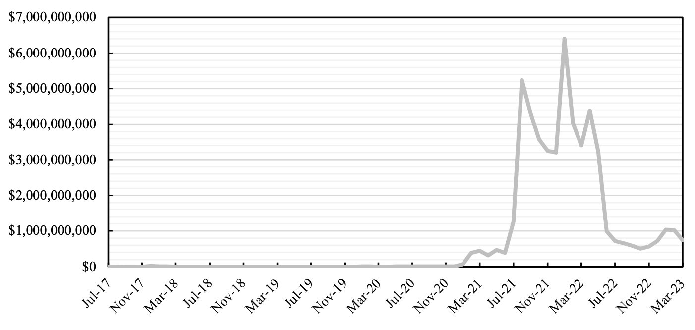
   Fig. 1. Above is the graph of monthly NFT sales over the period described by the dataset. Prior to 2021, monthly NFT sales are not even discernible.

   As mentioned in the introduction, monthly NFT sales have fluctuated significantly in the market’s history. This fact is observable in Figure 1. Monthly sales were relatively insignificant prior to Q2 2021, then experienced a time of enormous growth in 2021 and 2022 and are currently a fraction of what they used to be at their peak.

   A notable statistic about monthly NFT sales is its degree of autocorrelation. Autocorrelation measures the correlation between data and a lagged version of that data over time. In other words, it describes the ability of a series to continue a trend established by past values of itself. A Durbin-Watson D-Statistic (DW) for the regression of NFT sales was calculated using the following formula, where êt represents residual and T is the number of observations (69 in this case). The D-Statistic ranges from 0 to 4, in which values closer to 0 indicate a positive autocorrelation and values closer to 4 indicate a negative autocorrelation. A D-Statistic of 2 indicates that no autocorrelation exists within the series.

   
   

   $$DW=\frac{\sum_{t=2}^{T}\left({\hat{e}}_t-{\hat{e}}_{t-1}\right)^2}{\sum_{t=1}^{T}\left({{\hat{e}}_t}^2\right)}$$

   The Durbin-Watson D-Statistic for monthly NFT sales was calculated to be 0.2858. In accordance with standard interpretation, this result implies that NFT sales exhibit strong positive autocorrelation. This means that an increase in NFT sales for one month is very likely to lead to a proportional increase in total sales for the next month; the opposite effect occurs during a decrease in sales. The major takeaway from the Durbin-Watson D-Statistic is that NFT sales are very “trendy” and subject to streaks of increasing or decreasing sales. Thus, identifying the beginning of one of these streaks could be extremely important in predicting a longer-term trend for NFT sales. This streaky nature led to the hypothesis that changes in the average NFT consumer’s behavior may significantly precede changes in NFT sales.

   To better understand the average NFT consumer’s behavior over time, two simple metrics on a monthly time frame were calculated. The Buyer Activity Metric (BAM) represents the average number of NFT transactions made per buyer; it was calculated by dividing the number of transactions by the number of buyers each month. The Buyer Valuation Metric (BVM) represents the average USD value of NFTs purchased per buyer. The BVM was calculated by dividing monthly NFT sales by that month’s number of buyers. These metrics provide important information on how the characteristics of the average NFT consumer have changed over time and how NFT consumers respond to shifting market conditions. Figure 2 visualizes both metrics over the period accounted for in the dataset. Interestingly, while significant fluctuations are present in each metric, they are much less severe than those of NFT sales. This is especially apparent when comparing the monthly percent changes in values of the BVM, the BAM, and NFT sales.10

   
   

   Buyer Valuation Metric and Buyer Activity Metric, 2017-2023

   

   
   

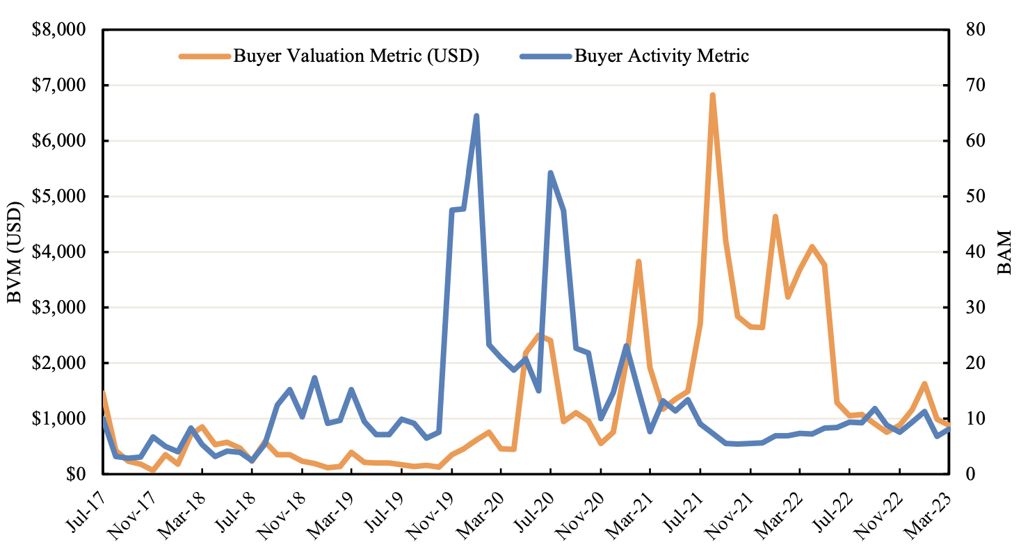
   Fig. 2. Dual-axis visualization of the Buyer Valuation Metric and the Buyer Activity Metric. The two metrics are not correlated (R2 = 0.0017).

   
   

   To investigate the forecasting ability of the BVM and the BAM on total monthly NFT sales, a Vector Autoregression (VAR) framework was constructed. A VAR framework can analyze the dependencies between several variables and has been used for financial analysis in prior NFT research.11 In a VAR model, the vector of one variable is modeled as being dependent on the lags of itself and those of the other variables included in the model. To meet the conditions for the VAR model, the time-series for the variables were made stationary. This was done by converting BVM, BAM, and NFT sales data to their logarithmic forms and then differencing once. Augmented Dickey-Fuller (ADF) Tests for proving stationarity are observable in Table 1.1 and Table 1.2.12 A Johansen test for cointegration also revealed that zero cointegrating relationships between the original time series existed, further ensuring the suitability of the VAR model.13 With the three log-differenced and non-cointegrated variables, the equation for the VAR model is as follows.

   
   

   $$\left[\begin{matrix}{BVM}_t\\{BAM}_t\\{NFT\ sales}_t\\\end{matrix}\right]=a_0+A_1\left[\begin{matrix}{BVM}_{t-1}\\{BAM}_{t-1}\\{NFT\ sales}_{t-1}\\\end{matrix}\right]+\cdots+A_4\left[\begin{matrix}{BVM}_{t-4}\\{BAM}_{t-4}\\{NFT\ sales}_{t-4}\\\end{matrix}\right]+\left[\begin{matrix}\varepsilon_{1,t}\\\varepsilon_{2,t}\\\varepsilon_{3,t}\\\end{matrix}\right]$$

   
   

   The appropriate number of lags for the VAR model was determined to be 4 using the Akaike information criterion.14 a0 is the vector of constant intercept terms from the three variables in the VAR model. A1 through A4 are the coefficients of the lags included in the VAR (lags 1 through 4). The vector of epsilons represents error. The creation of this VAR model is necessary because it is the foundation for the post-estimation tool used to analyze the predictive abilities of the BVM and BAM.

4. Results and Discussion

   The principle post-estimation tool used to assess the VAR model was the Granger-causality hypothesis test. Granger-causality is a method of econometric analysis developed by Clive Granger in the 1960s and widely applied since.15 The null hypothesis for a Granger-causality test is that one variable in the underlying VAR model does not “Granger-cause” another—meaning that the values of one variable do not precede the values of another. Granger-causality tests are useful for determining the predictive abilities of variables in a VAR model. The results for the Granger-causality tests are summarized in Table 1.

   
   

   Table 1. Granger-Causality Tests for Metrics, NFT Sales

   
   

   Response Variable	Explanatory Variable	Chi-Squared Statistic	p-value
   NFT Sales	BAM	25.187	0.000***
   	BVM	37.502	0.000***
   BAM	NFT Sales	0.0883	0.999
   	BVM	4.6882	0.321
   BVM	NFT Sales	0.2703	0.992
   	BAM	0.4600	0.977
   *** p < 0.01; ** p < 0.05; * p < 0.1.

   
   

   Changes in each consumer-oriented metric—the BVM and the BAM—Granger-cause changes in NFT sales. Since a lag of four was used in the underlying VAR model, changes in each metric are interpreted as preceding changes in NFT sales by up to four months. Furthermore, the Granger-causation of the BVM on NFT sales and the BAM on NFT sales are unidirectional. These Granger-causality tests are substantial evidence of the lagged effect that consumers have on the NFT market. When consumers’ behaviors change, one can expect the amount in sales in the NFT market to later change accordingly. It is reiterated that these findings are meaningful because the data met all conditions for the VAR model: the original variable series are not cointegrated and the once-differenced logarithmic series are stationary.

   Of course, there is the possibility that the individual components of the BAM and BVM (number of transactions, number of buyers, and sales) may be driving the metrics’ relationships to NFT sales. In particular, the “number of buyers” variable may be motivating the Granger- causal relationships present for both the BAM and BVM, since number of buyers appears in the definition of both variables. To examine this possibility, another VAR model is constructed of three log-differenced variables: NFT sales, number of buyers, and number of transactions. Although there is one cointegration present between these variables, a Granger-causality test is still carried out for the sake of comparison against the initial tests; the log-differenced data are stationary and the Akaike information criterion identifies the optimal lag of 3 months.16

   While the number of buyers in the NFT market do Granger-cause NFT sales, this relationship is bidirectional. In fact, monthly NFT sales appear to have a greater predictive ability for the number of buyers (and transactions) than the other way around. The bidirectionality in these results could be due to the cointegration present between the variables, which confounds the “predictive” ability of the number of buyers. For these reasons, the number of monthly buyers in the NFT market is of less value than the BAM or BVM in signaling directional shifts in NFT sales. This is because, as seen in the discrepancies of p-values within Table 3, the BAM and BVM have strongly unidirectional Granger-causalities with NFT sales. Furthermore, the metrics’ Granger-causalities exist at lower p-values than that of the number of buyers, and it should also be reiterated that the BAM and BVM are not cointegrated or correlated despite both metrics using data on the number of buyers. All of these aspects lead to the conclusion that the predictive ability of the BAM and BVM are not dominated by that of the number of buyers, and that the BAM and BVM have unique Granger-causal relationships to the NFT market’s sales.

   
   

   Table 2. Granger-Causality Tests for Components of Metrics, NFT Sales

   
   

   Response Variable	Explanatory Variable	Chi-Squared Statistic	p-value
   NFT Sales	Buyers	10.004	0.019**
   	Transactions	2.7147	0.438
   Buyers	NFT Sales	33.824	0.000***
   	Transactions	2.2228	0.527
   Transactions	NFT Sales	35.996	0.000***
   	Buyers	12.616	0.006***
   *** p < 0.01; ** p < 0.05; * p < 0.1.

   
   

   It should be acknowledged that, while the BVM and the BAM may have some predictive abilities on NFT sales, using a VAR model to precisely forecast NFT sales is unadvisable. This is due to the fundamentals of the NFT market—it is driven by speculative investment. Consequently, investors are drawn to NFTs because of the potential for extremely high returns and are willing to accept extremely high volatility as a result.17 So, despite being positively autocorrelated, monthly NFT sales are subject to sudden and extreme changes in directional trend. A VAR forecast for sales will likely be impractical, as the NFT market simply experiences too much volatility for autoregressive modeling to account for. Still, the results of the Granger- causality tests are quite beneficial to consumers’ understandings of the NFT space. By consulting the BVM and BAM, shifts in the market can be identified months in advance. This type of prediction is important considering the degree of autocorrelation inherent to NFT sales; a shift in the market will likely extend to the longer term. As it relates to NFT investors, being able to predict the health of the overall NFT ecosystem is a valuable tool. One investment- application of these findings relates to market-entry times, as investors will want to enter a speculative investment when there is sustained momentum surrounding the industry—the BAM and BVM can certainly help indicate when this is the case.

   
   

5. Plausible Theoretical Explanations of Results

   With the practical applications outlined, it is important to begin trying to understand why changes in the BVM and BAM precede changes in NFT sales. Several possible explanations for the Granger-causal relationships are discussed below, although this is done in theoretical fashion; additional research should be undertaken to explore each of these hypotheses.

   1. NFT Whales Initiating Market Trends—Although lagged changes in the average consumer’s behavior significantly affect sales, perhaps this average is inflated by a very small number of high-value users. Previous research has established the presence of “NFT whales”— the top 0.1% of NFT traders that hold 5% of all NFT tokens which account for nearly 20% of the NFT market’s value.18 Furthermore, Park et al. note that only a few NFT collections account for most of the NFTs market’s capitalization. These influential collections are also more likely to be minted by whales. This significant advantage in setting NFT valuations is another clear sign of whales’ impacts on the market, and they may even initiate market trends because of these early connections to especially popular collections. The longitudinal study concludes its analysis of NFT whales by stating that, because of their enormous impacts on the NFT market, they also dictate market sentiment. As mentioned prior, it could be that the BAM and BVM model disproportionately reflect the purchasing behavior of whales. Changes in the BAM and BVM would hence indicate changes in whale activity and valuation. Continuing with this interpretation, Granger-causal relationships within this paper’s VAR model would support the idea that whales drive the NFT market. This effect is surely exaggerated by NFT sales’ strong degree of positive autocorrelation, which could be attributed to trends set by whales in the first place. To conclude, the results of this study may advance the idea that Park et al. presented. Consumer behavior has a lagged and quantitative influence on NFT sales; it may also be representative of whales and the trends they begin.

   2. Delayed Effects on Monthly Sales Attributed to NFT Holding Times—Holding times of NFTs may also be related to the predictive abilities that consumer behavior has on NFT sales. The basis for this theory lies in the fact that when the number or dollar-amount of NFTs purchased by the average consumer experiences a change, NFT sales typically experience a change within four months later. As discussed previously, this effect could be from a combination of several factors (whales’ tendencies to own high-value NFT collections and their influence on markets). Regardless of its cause, the four-month lagging period warrants further research into the typical holding times of high-value NFTs. This is because the holding times of high-value NFTs may explain the four-month Granger-causal lag. For example, if a high- value NFT collection experiences its primary sales during “month one” and is then mostly resold four months later, one would expect the BAM and BVM to increase during “month one” and NFT sales to increase during “month five.” The notion that a large amount of high-value NFTs would be resold in a short period of time makes logical sense, since high-value NFTs are likely to be owned by a small number of whales to begin with. If whales need to liquidate their expensive wallets, or if they are simply no longer interested in a particular collection, multiple high-value NFTs could be sold at once. Not only are whales most prone to owning high-value NFTs, but they also hold these high-value NFTs for relatively long periods of time. The range, mean, and mode of the distribution of whales’ high-value NFT holding times are all greater than those of the bottom 99.9% of NFT traders as Park et al. discovered. Since whales have a significant influence on the market overall, whales’ holding times of high-value NFTs could also influence NFT sales. This impact should be investigated independently of this paper’s findings since it may have implications for the NFT market’s vitality. For example, a sudden decrease in whales’ holding times could create selling pressure in the market. This would lead to a troublesome seller-dominated environment in which a relatively low number of buyers could drive NFT prices downward as sellers try to liquidate their holdings. Clearly, this scenario would be devastating for the NFT market, and it is not far-fetched either. The entirety of April 2023 was concerningly seller-dominated and the market has been mostly slumped since.19 However, if the Granger-causal relationships are indeed attributed to whales’ holding times, consumer-oriented metrics could provide warnings of future seller-dominated periods.

6. Conclusion

The ability to forecast changes in total NFT sales is important considering the market’s extreme volatility over the past years. Therefore, research was conducted to determine whether consumer behavior in the NFT market has a delayed effect on NFT sales. Understanding what precedes fluctuations in market vitality is important. Econometric discoveries would lead to a deeper understanding of the NFT market’s nature, while consequent forecasting tools would provide practical benefits for NFT consumers/traders.

To begin, two consumer-oriented metrics were created using NFT data: the Buyer Valuation Metric (BVM) and the Buyer Activity Metric (BAM). A three-variable vector autoregression (VAR) model was created using these two metrics and NFT sales data. It was discovered that changes in each of these metrics Granger-cause changes in the market’s monthly NFT sales. It can therefore be concluded that fluctuations in consumer behavior precede gains or losses in the NFT market.

These findings have several implications, the first of which relates to NFT consumers. Given that NFT sales are simultaneously volatile and highly autocorrelated, the BVM and BAM are important indicators to users and investors alike. The two metrics may be useful as predictors for significant shifts in the market’s sales since the direction of these shifts will likely extend to the longer term. Secondly, metrics that quantify consumer behavior could be used to evaluate threatening developments in the NFT ecosystem. A recent cause for concern has been seller-dominated market conditions. Because of the NFT market’s underlying characteristics, a seller-dominated market could decrease NFT sales quickly and extremely. With further investigative research, it is possible that consumer-oriented metrics could give ample warnings and assessments of such tumultuous circumstances.

Author Contributions

Stoyan R. Angelov performed the entirety of the econometrics and manuscript-writing for this article. No other authors contributed to this article.

Conflict of Interest

The authors declare that they have no known conflicts of interest as per the journal’s Conflict of Interest Policy.

References

1 Browne, R. “Trading in NFTs Spiked 21,000% to More Than $17 Billion in 2021, Report Says,” CNBC (10 March 2023) https://www.cnbc.com/2022/03/10/trading-in-nfts-spiked-21000percent-to-top-17-billion-in-2021-report.html.

2 No Author. “NFT Market Reports.” Nonfungible.com (accessed 5 April 2024) https://nonfungible.com/reports.

3 White, J. T., Wilkoff, S., Yildiz, S. “The Role of Media in Speculative Markets: Evidence from Non-Fungible Tokens (NFTs)” Social Science Research Network http://dx.doi.org/10.2139/ssrn.4074154.

4 Garay, J., Kiayias, A., Leonardos, N. “The Bitcoin Backbone Protocol with Chains of Variable Difficulty,” Cryptology ePrint Archive (accessed 18 May 2024) https://eprint.iacr.org/2016/1048.pdf.

5 Wang, Q., Li, R., Wang, Q., Chen, S. “Non-Fungible Token (NFT): Overview, Evaluation, Opportunities and Challenges,” arXiv (accessed 18 May 2024) https://doi.org/10.48550/arXiv.2105.07447.

6 Taherdoost, Hamed. “Non-Fungible Tokens (NFT): A Systematic Review,” Information 14.1 26 (31 December 2022) https://doi.org/10.3390/info14010026.

7 Nadini, M. et al. “Mapping the NFT Revolution: Market Trends, Trade Networks, and Visual Features” Scientific Reports 11 20902 (22 October 2021) https://doi.org/10.1038/s41598-021-00053-8.

8 CryptoSlam occasionally updates its NFT market dataset. For access to the 5 April 2023 version of the dataset used in this research, please contact the author of this article.

9 No Author. “NFT Global Sales Index” CryptoSlam (accessed 5 April 2023) https://www.cryptoslam.io/nftglobal?timeFrame=month.

10 See Appendix A, Figure 1.1 and Figure 1.2.

11 Lennart, A. “The Non-Fungible Token (NFT) Market and its Relationship with Bitcoin and Ethereum” SSRN (6 June 2021) http://dx.doi.org/10.2139/ssrn.3861106.

12See Appendix B, Table 1.1 and Table 1.2.

13 See Appendix B, Table 1.3.

14 See Appendix B, Table 1.4.

15 Seth, A. “Granger causality,” Scholarpedia 2.7 1667 https:/doi.org/10.4249/scholarpedia.1667.

16 See Appendix B, Tables 2.1, 2.2, and 2.3.

17 Kong, D., Lin, T. “Alternative Investments in the Fintech Era: The Risk and Return of Non-fungible Token (NFT),” SSRN (26 June 2023) http://dx.doi.org/10.2139/ssrn.3914085.

18 Park, N. et al. “A Deep Dive into NFT Whales: A Longitudinal Study of the NFT Trading Ecosystem,” arXiv (2 Feb 2023) https://doi.org/10.48550/arXiv.2303.09393.

19 Lyons, C. “NFT Markets Are Out of Balance, with Sellers Dominating,” Cointelegraph (27 April 2023) https://cointelegraph.com/news/nft-markets-are-out-of-balance-with-sellers-dominating.

Appendix A: Monthly Percent Changes of BVM, BAM, NFT Sales

The equation below was used to calculate the monthly percent changes of each metric and of NFT sales. Refer to Figures 1.1 and 1.2 for summary statistics on the monthly volatilities for the BAM, the BVM, and NFT sales. Please note that outliers are not visible in Figure 1.1.

$$Percent\ {Change}_{{Month}_{n+1}}=100\bullet\left|\frac{{Month}_{n+1}-{Month}_n}{{Month}_n}\right|$$

Monthly Percent Change of Buyer Activity and Buyer Valuation Metrics

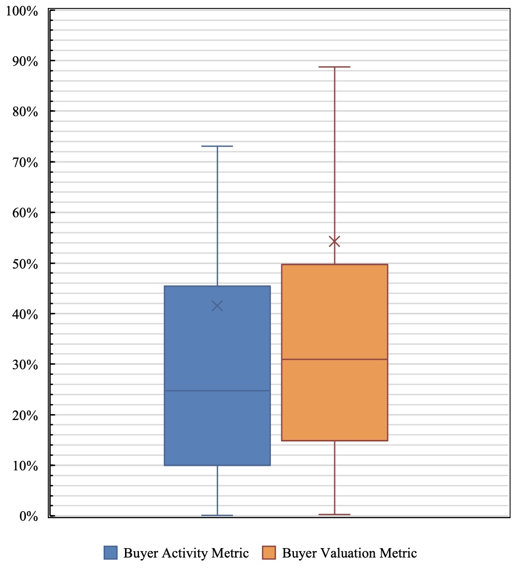
Fig. 1.1. Box and whisker plots of the monthly percent changes of the Buyer Activity Metric and Buyer Valuation Metric. Outliers are not visible for the purpose of visualization clarity.

Monthly Percent Change of NFT Sales

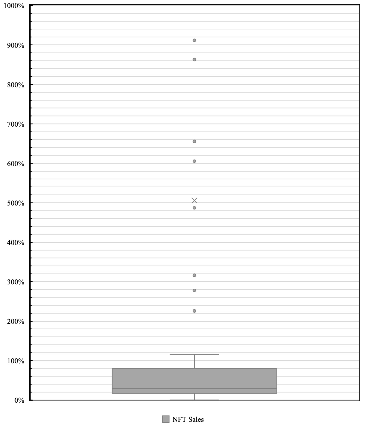
Fig. 1.2. Box and whisker plot of the monthly volatilities NFT sales. Outliers are made visible to illustrate the extreme degree of volatility. One may also note that the mean volatility is much greater than the median volatility, indicating an extreme skew.

Appendix B: Testing Conditions for VAR Mode with Metrics

Table 1.1. ADF Tests for Logarithmic Data

Table 1.2. ADF Tests for Logarithmic-Differenced Data

Table 1.3. Johansen Test for Cointegration

Table 1.4. AIC-based Lag-order Selection

Appendix C: Testing Conditions for VAR Model with Components of Metrics

Table 2.1. ADF Tests for Logarithmic-Differenced Data

Table 2.2. Johansen Test for Cointegration

Table 2.3. AIC-based Lag-order Selection